Home About

Theory: ParticleFlow

The two-dimensional model ParticleFlow simulates flow in a rectangular domain. A key purpose of the ParticleFlow model is to illustrate how heterogeneities in hydraulic properties cause the spatial spreading of fluid particles. This spreading is analogous to macro-scale solute dispersion.

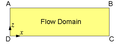
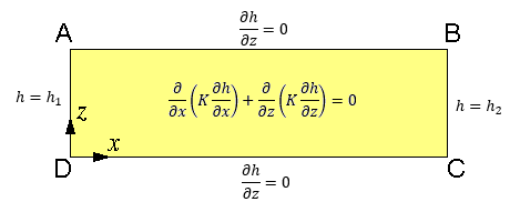
The rectangular flow domain is assumed to be bounded on the left and right sides (AD and BC) by specified head boundaries, and on the top and bottom (AB and DC) by no-flow boundaries. Assuming that the head along AD is higher then the head along BC, the average flow is from left to right.

The rectangular flow domain could represent either a vertical section or a horizontal plane.

ParticleFlow flow domain

Steady-state flow of ground water in the domain is governed by the equation

ParticleFlow flow equation

where h is hydraulic head, K is hydraulic conductivity, and x and z are the Cartesian coordinates. The boundary condition along AD is

ParticleFlow boundary condition at left side

where h1 is a constant. The boundary condition along BC is

ParticleFlow boundary condition at right side

where h2 is also a constant. The boundary conditions along AB and DC are both

ParticleFlow no-flow boundary
ParticleDrive mathematical problem

ParticleFlow solves the above equations by the finite-element method.

The flow domain is represented by a rectangular mesh composed of square cells, each is divided into two triangular elements

Linear basis functions are used to formulate the finite-element formulation.

ParticleFlow finite-element mesh

After solving for hydraulic head h, the x and y components of the groundwater velocity vector are computed by

ParticleFlow groundwater velocity computation

where n is porosity. The velocity vectors are used for calculating flow paths and the advective movement of fluid particles.

In a flow field with nonuniform velocity, a cloud of fluid particles will tend to spread. This spreading can be described by the spatial variance (in the x and z directions) of particle positions, defined as

ParticleFlow spatial variance

where N is the total number of fluid particles, xi and zi are the x and z coordinates of the i-th particle, xc and zc denote the x and z positions of the center of mass, defined as

ParticleFlow center of mass

If each fluid particle is assumed to carry a fixed amount of solute mass, then particle spreading is analogous to macro-scale solute dispersion. In the macro-dispersion approach, the small-scale variation of velocity is not explicitly simulation. Instead, solute spreading is characterized by a dispersion tensor. If dispersion process is Fickean, the plot of the spatial variances Sxx and Syy versus time show straight-line relations. In this case, the components of the dispersion tensor can be estimated by

ParticleFlow dispersion