How to Use ParticleFlow

Running ParticleFlow involves five steps, as described below. To begin each step, click the corresponding button at the top of the window.

At Step 4, two options are available. Follow Step 4a to compute flow paths, or Step 4b to set up fluid particles.

Step 4a is followed by Step 5a (animate flow paths). Step 4b is followed by Step 5b (animate particle movement).

Step 1: Specify the mesh and hydraulic gradient

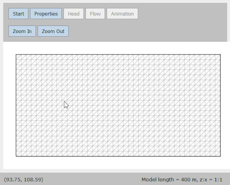
Click the "Start" button.
Enter the size of a square element, number of rows and column, and average hydraulic gradient. For example, if the element size is 10 m, and there are 40 columns and 20 rows, the grid will be 400 m by 200 m. A typical hydraulic gradient might be 0.001.
Click OK.

The program generates a rectangular mesh and then splits each square element into two triangular elements

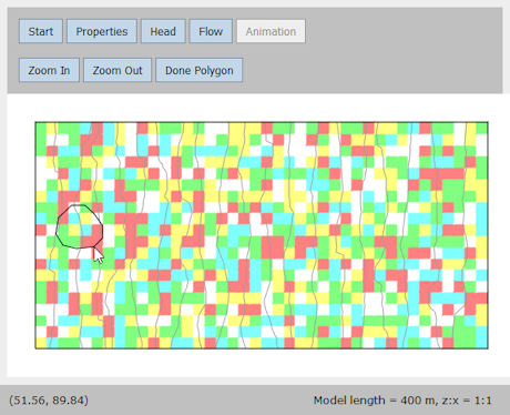
Note that the x and z coordinates of the cursor are shown at the lower left corner of the window.

ParticleFlow program window during Step 1

Step 2: Assign hydraulic properties

Click the "Properties" button.
Five sets of hydraulic conductivity (m/s) and porosity (%) values are available for assignment to model elements. Each set is represented by a color. Default values are initially provided, but users may alter any or all of these values in the edit boxes

Two options are now available. To randomly assign hydraulic conductivity and porosity values to the grid, click the "Randomize" check box and then click "OK". Each pair of triangle elements (forming a square) will be randomly assigned one of five colors corresponding to five sets of hydraulic conductivity and porosity values

Alternatively, properties can be manually assigned to the grid as follows:

Click on a color icon to select the corresponding property values.
Click "OK"
Draw a polygon to enclose those elements to be assigned the selected property values. A polygon is drawn by clicking at its vertices.
To finish drawing the polygon, double click the last vertex.

Repeat the above steps to assign hydraulic properties to other zones in the aquifer.

ParticleFlow program window during Step 2 (option 1)

ParticleFlow program window during Step 2 (option 2)

Step 3: Compute hydraulic head

Click the "Head" button.
Select the number of contour intervals to be drawn.
Click "Compute."

When the computation is finished, head contours are displayed

ParticleFlow program window during Step 3

Step 4a: Compute groundwater flow paths

Click the "Flow" button.
Select "Flow path tracking".
Select the direction of flow path tracking.
Click OK.
Click anywhere in the flow domain to track the flow path from that point in the direction(s) specified above.
Click on additional points in the flow domain to track additional flow paths.

ParticleFlow program window during Step 4a

Step 4b: Set up fluid particles

Click the "Flow" button.
Select "Particle movement".
Enter the initial particle spacing (in meters). As a general guide, use a spacing that is between 1/100 and 1/1000 of the model domain length.
Click OK.
Draw a polygon to outline the initial location of a cluster of fluid particles. Keep the polygon relatively small to avoid having too many particles.
After the polygon is drawn, it will be filled with particles at the prescribed spacing.
(Optional) Draw additional polygons to create additional clusters of particles.

ParticleFlow program window during Step 4b

Step 5a: Animate flow paths

Click the "Animation" button.
Set the animation speed by specifying the amount of travel time (in days or years) that is equal to 1 second of animation time.
Set the animation smoothness by specifying the number of frames per second. (The default setting of 10 frames per second is usually adequate.)
Click OK.
To start the animation, click anywhere inside the window, below the buttons.
Additional clicks alternately freeze and unfreeze the animation.

Travel time is shown at the bottom of the window.

ParticleFlow program window during Step 5a

Step 5b: Animate particle movement

Click the "Animation" button.
Set the animation speed by specifying the amount of travel time (in days or years) that is equal to 1 second of animation time.
Set the animation smoothness by specifying the number of frames per second. (The default setting of 10 frames per second is usually adequate.)
Local dispersion may be added by specifying non-zero values for longitudinal and transverse dispersivity (in m). Local dispersion represents spreading caused by heterogeneities at subgrid level, and is simulated by adding a small random perturbation to the particle movement at each time step. As a general rule, the local dispersivities should be less than the element size. To turn off local dispersion (that is, to simulate purely advective transport), set the dispersivities to zero.
Set the options to show the center of mass, standard deviations, or plots of spatial variance versus time by checking or unchecking the option boxes.
Click OK.
To start the animation, click anywhere inside the window, below the buttons.
Additional clicks alternately freeze and unfreeze the animation.

Travel time is shown at the bottom of the window.

If activated, the center of mass in the x and z directions are respectively indicated by blue and green arrow heads. The distance spanned by the specified number of standard deviations (on both sides of the center of mass) is indicated by blue and green lines.

If activated, the plots of spatial variance (Sxx and Szz) versus time are shown next to the model domain. To see these plots, it might be necessary to increase the size of the window or reduce the size of the model domain by zooming out.

ParticleFlow program window during Step 5b